Track 2 Memory-Bandwidth Penalty
Version 1.0 · Last Updated: October 9, 2026
Table of Contents
- 1. Motivation
- 2. Additive Bandwidth Penalty
- 3. Theoretical Estimate Versus Profiler Measurement
- 4. Participant Reporting Requirement
- 5. Computing Theoretical Memory-Bandwidth Use
- Appendix: Worked Examples
- A. Single Full Conv1D Layer
- B. Depthwise-Separable Conv1D Layer
- C. ConvNeXt 1D Block
- D. ResNet BasicBlock: Two 3x1 Conv1D Layers
- E. ResNet Bottleneck Block
- F. Residual Vector Quantization Block
- G. Recurrent GRU Layer
- H. Strictly Causal Streaming Self-Attention with KV-Cache
- I. Rotary Positional Embedding (RoPE)
Purpose: Define an additive memory-bandwidth penalty for LRAC 2.0 Track 2.
Primary metric: Total theoretical persistent-tensor memory bandwidth in MB/s of processed audio.
Penalty policy: No penalty up to 50 MB/s; logarithmic penalty above 50 MB/s; maximum penalty of 15 points at 1 GB/s.
1. Motivation
Low-end mobile devices are an important deployment target for neural audio codecs. They have limited memory bandwidth, smaller caches, tighter thermal envelopes, and less headroom for background workloads. A codec that sounds good on a workstation can still be impractical if its streaming implementation repeatedly moves large weight, activation, state, or cache tensors through memory.
The first edition of the Low-Resource Audio Codec (LRAC) Challenge already constrained codecs along several practical axes, including computational complexity, latency, and bitrate. It did not, however, include a direct constraint on model size, memory bandwidth, or peak memory usage. LRAC 2.0 Track 2 encourages low-memory codec designs through a 1.5 million parameter eligibility cap and an additive memory-bandwidth penalty applied to the aggregated subjective quality and intelligibility score.
Running a codec on a fixed reference platform and measuring its real-time factor (RTF) would capture the combined effects of computation, memory behavior, and implementation on that platform. RTF is useful for checking whether the codec keeps pace with incoming audio, although it does not alone establish that every streaming step meets the latency limit. We do not use it for Track 2 scoring because participants would have to port and tune their codecs for one system. That would be a substantial, uneven engineering effort, and rankings would depend partly on implementation choices and toolchains rather than codec architecture.
Memory bandwidth consumption is not the sole memory constraint for codecs running on low-resource devices; model size and peak memory can also be limiting. However, memory bandwidth consumption is one of the most important constraints for streaming inference and is closely related to model size and streaming state. It is therefore a simple, auditable first memory-related metric for the challenge, without turning the score into a weighted combination of many resource terms.
Parameter count describes model size, while the bandwidth metric captures how often each layer’s weights are read at its streaming frame rate. It also counts traffic from streaming convolution state, recurrent hidden state, and the attention key-value cache (KV-cache); the KV-cache can grow with context length without adding parameters. Two models with identical parameter counts can therefore differ substantially in memory bandwidth, which is why we use memory bandwidth rather than mere parameter count.
Peak memory is especially important because it behaves like a hard deployment constraint: if the required peak memory exceeds the available memory budget, the implementation may fail outright rather than merely run more slowly. Peak memory is not a second score axis. Adding it would make the penalty formula more complex and would increase the burden on participants to compute another metric accurately. Peak-memory estimates are also often driven by a single worst-case layer, temporary buffer, or tensor-lifetime/buffer-reuse assumption, which can make them noisier than an accumulated bandwidth estimate and could introduce unnecessary noise into challenge rankings.
LRAC 2.0 has two tracks. Track 1 ranks transparency codecs on aggregated subjective quality and intelligibility alone. Track 2 ranks memory-efficient transparency codecs after applying the additive memory-bandwidth penalty introduced in the next section, subject to its 1.5 million parameter cap. This keeps progress toward transparency visible while also motivating architectures that achieve comparable quality with lower theoretical memory bandwidth.
2. Additive Bandwidth Penalty
For Track 2, let S be the aggregated subjective quality and intelligibility score, with S in [0, 100]. Let B be the theoretical memory-bandwidth demand of the submitted codec operating at its maximum supported bitrate: the counted logical traffic for processing one second of audio in real time, expressed in MB/s. B is neither measured DRAM traffic nor a device’s bandwidth capacity. Participants should report B for the complete codec network, including encoder, quantizer, and decoder accesses on the transmit and receive sides. The effective score after the bandwidth penalty is:
S_effective = max(0, S - P(B))
For LRAC 2.0 Track 2, the additive penalty is zero below the bandwidth threshold, increases logarithmically above it, and reaches its maximum at 1 GB/s:
P(B) = 0                                                   for B <= B0
P(B) = P_max * ln(B / B0) / ln(Bsat / B0)                  for B0 < B < Bsat
P(B) = P_max                                               for B >= Bsat
For the challenge, B0 = 50 MB/s, Bsat = 1000 MB/s, and P_max = 15 score points.
The logarithmic ramp charges an equal absolute penalty per doubling of bandwidth. For example, the 50 -> 100 MB/s increase costs the same number of points as the 500 -> 1000 MB/s increase. This matches the intuition that relative bandwidth growth is what matters and keeps the policy simple to explain.
This additive form also avoids the bias introduced by a multiplicative correction. With a multiplier, two systems using the same bandwidth lose different numbers of score points: the higher-quality system loses more points in absolute terms. With an additive penalty, both systems lose the same number of points for the same bandwidth. A low-quality high-bandwidth system loses a larger fraction of its score than a high-quality one, which is generally the more defensible direction.
P_max is fixed at 15 points for the LRAC 2.0 Track 2 challenge. Each bandwidth doubling between 50 MB/s and 1000 MB/s therefore costs about 3.47 points, and the penalty remains 15 points above 1000 MB/s. Figure 1 shows the penalty curve, and Table 1 lists values at successive doublings of the 50 MB/s threshold and at the 1000 MB/s cap.
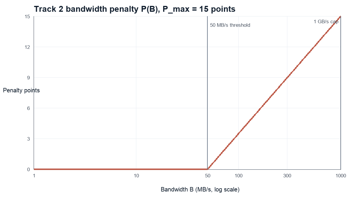
Figure 1. Track 2 additive bandwidth penalty with P_max fixed at 15 points.
Table 1. Track 2 penalty at bandwidth doublings and the 1000 MB/s cap.
| Bandwidth B | Penalty with P_max = 15 |
|---|---|
| 50 MB/s | 0.00 |
| 100 MB/s | 3.47 |
| 200 MB/s | 6.94 |
| 400 MB/s | 10.41 |
| 800 MB/s | 13.88 |
| 1000 MB/s | 15.00 |
3. Theoretical Estimate Versus Profiler Measurement
The official challenge metric should use a theoretical architecture-level estimate rather than a profiler-derived hardware measurement. Theoretical bandwidth is reproducible from the network description, can be checked from an analytical model-design sheet, and does not depend on a participant’s GPU, CUDA version, kernel library, batching strategy, or profiling tool.
Depending on the platform, CPU and GPU profilers can measure memory-system behavior such as DRAM traffic, cache activity, and achieved bandwidth. Those measurements are useful for implementation optimization, but they measure implementation-dependent traffic rather than the challenge’s theoretical bandwidth estimate. Table 2 summarizes the measurement issues behind this choice.
Table 2. Reasons profiler measurements are unsuitable for primary scoring.
| Issue | Why it complicates profiler-based scoring |
|---|---|
| Hardware specificity | Profiler results are tied to a specific hardware and software stack, while challenge evaluation should be hardware agnostic and comparable across deployments. |
| Cache and fusion effects | DRAM traffic may be below logical traffic when weights stay in cache or fused kernels avoid intermediate writes. |
| Implementation overhead | DRAM or L2 traffic may be above theory because of layout conversions, temporary buffers, padding or framing copies, or non-fused kernels. |
| Batching and amortization | Profiling multiple streams together can spread weight reads across them. GPU batching may amortize weight loads, while CPU execution may reuse cached weights across streams; these measurements may differ from a single-stream run. |
Profiler measurements should be allowed as supplementary evidence and for engineering validation. They should not be the primary challenge score because they are implementation- and device-dependent. The mandatory score input should be theoretical logical memory bandwidth, computed from the model architecture and submitted with formulas.
4. Participant Reporting Requirement
Track 2 participants should submit a detailed analytical model-design sheet summarizing the network layer by layer. The sheet should make the bandwidth computation auditable and should also report compute complexity and latency. For the bandwidth score, all counted tensor values use 2 bytes/value regardless of the implementation’s weight precision, so weight dtype is not a required field. The bandwidth calculation does not require participants to publish source code or model weights. Table 3 lists the fields participants should provide.
The completed baseline analytical model-design sheets provide worked examples for Track 1 and Track 2. In particular, the Track 2 sheet demonstrates how the bandwidth convention on this page is applied to a complete codec. The sheets are specific to the baseline VoCodec architecture and are not general templates; participants must adapt the analytical calculations to their own systems. See the Baseline guidance for further context.
Table 3. Fields required in the Track 2 participant analytical model-design sheet.
| Required field | Description |
|---|---|
| Layer/block name | Architecture component, repeated count, and streaming or causal behavior. |
| Tensor dimensions | Input, output, hidden/intermediate, codebook, KV-cache, and state dimensions. |
| Layer frame rate | Streaming frame rate F_l for each layer or block. Encoder strides and decoder transposed convolutions may produce different rates across layers. |
| Compute complexity | MACs or FLOPs per audio second, with formulas. |
| Latency | Total algorithmic and buffering latency, at most 30 ms, with state and cache assumptions. |
| Parameter count | Unique trainable parameters of the complete codec, including encoder, quantizer, and decoder; identify nontrainable model buffers separately when included in the parameter cap. |
| Bandwidth terms | Weight/codebook and persistent state/cache bandwidth with formulas. Normal activation traffic is not part of the primary score. |
5. Computing Theoretical Memory-Bandwidth Use
The Track 2 metric counts model parameters, codebooks, persistent model buffers, and streaming state or cache traffic. It excludes ordinary layer-boundary activations and is reported in decimal MB/s, where 1 MB = 1,000,000 bytes.
5.1 Assumptions and Simplifications
-
Weight-reload convention: count weight values once per layer frame at that layer’s frame rate. For RVQ, scan the full codebook on transmit and read only the selected embedding on receive.
-
Operating bitrate: compute B at the codec’s maximum supported bitrate. Use this single B to calculate one P(B), then subtract P(B) from the codec’s overall aggregated subjective quality and intelligibility score.
-
Persistent tensors only: the primary score includes weights, codebooks, persistent inference tensors (such as STFT windows), streaming state, recurrent hidden state, and attention KV-cache.
-
Intermediate activations: normal layer-to-layer activation traffic is set to zero, assuming streaming implementations keep adjacent activations cache-resident when the active working set fits cache.
-
Activation spill: extra reads and writes when intermediate activations move from registers or cache to slower memory. Excluded because this depends on tiling, working-set size, and cache behavior.
-
Precision: all counted values use b = 2 bytes/value regardless of weight precision. Weight quantization is outside this score; quantization of audio or learned embeddings remains in scope.
-
Tensor layout: count logical values as if stored contiguously; padding and layout overhead are not charged.
-
Scattered access: no extra charge is made for noncontiguous or data-dependent access patterns.
-
Sparsity: zeros in counted tensors receive no discount; reductions in tensor dimensions or state accesses do.
5.2 Memory Bandwidth Demand Computation
BW_challenge = BW_transmit + BW_receive
             = BW_parameters/codebooks/buffers + BW_persistent_state/cache
BW_layer = F_l * b * (P_l + R_l)
F_l is layer l’s streaming frame rate, and b is fixed at 2 bytes/value. P_l counts accessed parameters, codebooks, and persistent model buffers; R_l counts persistent state reads and writes separately. Shared parameters count once toward parameter count, but accesses on both sides enter B.
BW_intermediate_activations = 0
Normal intermediate activation traffic is zero by convention.
The core conversion is:
bytes = number_of_values * bytes_per_value
For each layer, multiply parameter bytes by its own streaming frame rate F_l. Strided encoder and transposed-convolution decoder layers may have different rates; total streaming latency must stay at or below 30 ms.
BW_W,l = |W_l| * b * F_l
Appendix: Worked Examples
The examples below use the fixed challenge convention of b = 2 bytes/value unless stated otherwise. In the formulas, F is the frame rate of the illustrated layer or block in frames/s. Unless otherwise stated, F = 100 frames/s. A complete codec must use each layer’s own frame rate, which can change across encoder and decoder stages. The totals use the primary persistent-tensor convention: normal intermediate activation traffic is not included. All MB/s values use decimal MB. Table 4 previews the bandwidth estimates developed below.
The convolution and attention examples use bias-free projections unless a bias is explicitly shown. A submitted codec must count the biases and other persistent tensors it actually accesses.
Table 4. Bandwidth estimates for the worked examples.
| Example | Approx. bandwidth |
|---|---|
| Single full Conv1D, C_in=C_out=256, K=5, dilation=3 | 66.8 MB/s |
| Depthwise-separable Conv1D, C=256, K=5 | 13.8 MB/s |
| ConvNeXt 1D block, C=192, M=216, K=7 | 17.4 MB/s |
| ResNet BasicBlock, C=192, K=3, two norms | 44.7 MB/s |
| ResNet Bottleneck, C=192, M=64, K=3, three norms | 7.55 MB/s |
| RVQ, C=192, D=8, R=6, N=1024 (both sides) | 15.8 MB/s |
| GRU, input D=256, hidden H=512 | 236.4 MB/s |
| Strict causal MHA with KV-cache, d=192, L=200 | 44.9 MB/s |
| RoPE, rotary dim=28, 4 heads, encoder and decoder | 0.0056 MB/s |
A. Single Full Conv1D Layer
This example estimates one strictly causal full Conv1D layer with dilation d = 3. C_in and C_out are its input and output channels, K is the number of kernel taps, F is this layer’s frame rate, and b is bytes/value. Table 5 lists the values used in the example.
Table 5. Inputs for the Single Full Conv1D Layer.
| Quantity | Value |
|---|---|
| Layer frame rate F | 100 frames/s |
| Input channels C_in | 256 |
| Output channels C_out | 256 |
| Kernel size K | 5 |
| Dilation d | 3 |
| Bytes/value | b = 2 |
1. Weight Bandwidth
A full Conv1D layer has K * C_in * C_out weights. Under the challenge convention, those weights are counted once per output frame of this layer.
N_W = K C_in C_out
    = 5 * 256 * 256 = 327,680 values
B_W = N_W b = 327,680 * 2 = 655,360 bytes = 0.65536 MB
BW_W = B_W F = 655,360 * 100 / 10^6 = 65.536 MB/s
2. Activation Convention
The input window and output frame are normal streaming activations. Under the primary challenge convention, they are assumed cache-resident and are not counted as external memory-bandwidth traffic.
BW_A,score = 0 MB/s
3. Streaming State Bandwidth
Dilation d spaces the K kernel taps across 1 + (K - 1)d input frames, so the causal layer retains (K - 1)d previous input frames. We count one read and one write of this entire state per output frame.
N_state = (K - 1)d C_in = 4 * 3 * 256 = 3,072 values
BW_state = 2 F b (K - 1)d C_in
         = 2 * 100 * 2 * 4 * 3 * 256
         = 1,228,800 bytes/s = 1.2288 MB/s
4. Total
BW_full-Conv1D = BW_W + BW_state
               = 65.536 + 1.2288 = 66.7648 MB/s ~= 66.8 MB/s
Table 6 summarizes the calculated bandwidth terms.
Table 6. Bandwidth breakdown for the Single Full Conv1D Layer.
| Term | Bandwidth |
|---|---|
| Weight reads | 65.536 MB/s |
| Streaming state | 1.2288 MB/s |
| Intermediate activation traffic | 0 MB/s |
| Total | 66.8 MB/s |
Result. One full Conv1D layer with C_in = C_out = 256, K = 5, and dilation d = 3 requires about 66.8 MB/s. Dilation increases the streaming-state term while leaving the number of weights unchanged.
B. Depthwise-Separable Conv1D Layer
This layer uses a temporal depthwise convolution followed by a 1x1 pointwise projection. C is the channel dimension, K is the depthwise temporal kernel size, F is the layer frame rate, and b is bytes/value. Table 7 lists the values used in this example.
Table 7. Inputs for the Depthwise-Separable Conv1D Layer.
| Quantity | Value |
|---|---|
| Layer frame rate F | 100 frames/s |
| Channel dimension C | 256 |
| Depthwise kernel size K | 5 |
| Pointwise projection | C -> C |
| Bytes/value | b = 2 |
1. Weight Bandwidth
The depthwise part has K * C weights. The pointwise part has C * C weights.
N_W = K C + C^2
    = 5 * 256 + 256^2 = 66,816 values
B_W = N_W b = 66,816 * 2 = 133,632 bytes = 0.134 MB
BW_W = B_W F = 0.134 * 100 = 13.4 MB/s
2. Streaming State Bandwidth
Only the temporal depthwise convolution needs streaming state.
BW_state = 2 F b (K - 1) C
         = 2 * 100 * 2 * 4 * 256
         = 409,600 bytes/s = 0.410 MB/s
3. Activation Convention
The input, depthwise output, and final output are normal streaming activations. They are assumed cache-resident and are not counted in the primary score.
BW_A,score = 0 MB/s
4. Total
BW_depthwise-separable ~= 13.4 + 0.410
                       ~= 13.8 MB/s
Table 8 summarizes the calculated bandwidth terms.
Table 8. Bandwidth breakdown for the Depthwise-Separable Conv1D Layer.
| Term | Bandwidth |
|---|---|
| Depthwise-conv weights | 0.256 MB/s |
| Pointwise-projection weights | 13.1 MB/s |
| Streaming state | 0.410 MB/s |
| Intermediate activation traffic | 0 MB/s |
| Total | 13.8 MB/s |
Result. The depthwise-separable layer is about 13.8 MB/s. The dominating term is the 1x1 pointwise-projection weight read.
C. ConvNeXt 1D Block
Assume a streaming ConvNeXt-style block: depthwise Conv1D, LayerNorm, Linear(C -> M), GELU, Linear(M -> C), and residual add. C is the input/output channel dimension, M is the intermediate expansion dimension, K is the depthwise temporal kernel size, F is the layer frame rate, and b is bytes/value. Table 9 lists the values used in this example.
Table 9. Inputs for the ConvNeXt 1D Block.
| Quantity | Value |
|---|---|
| Layer frame rate F | 100 frames/s |
| Input/output dimension C | 192 |
| Intermediate dimension M | 216 |
| Depthwise kernel K | 7 |
| Bytes/value | b = 2 |
1. Weight Bandwidth
The block has K * C depthwise weights plus two pointwise matrices, C * M and M * C.
N_W = K C + C M + M C = K C + 2 C M
    = 7 * 192 + 2 * 192 * 216 = 84,288 values
B_W = N_W b = 84,288 * 2 = 168,576 bytes = 0.169 MB
BW_W = B_W F = 0.169 * 100 = 16.9 MB/s
2. Depthwise Streaming State
The causal depthwise convolution retains K - 1 previous frames per channel.
BW_state = 2 F b (K - 1) C
         = 2 * 100 * 2 * 6 * 192
         = 460,800 bytes/s = 0.461 MB/s
3. Activation and LayerNorm Convention
Intermediate activations and LayerNorm statistics are assumed cache-resident and are not included in the primary score. LayerNorm scale and bias are parameters, so they are counted.
BW_A,score = 0 MB/s
BW_LN-params = F b (2 C)
             = 100 * 2 * (2 * 192) = 0.077 MB/s
4. Total
BW_ConvNeXt ~= 16.9 + 0.461 + 0.077
             ~= 17.4 MB/s
Table 10 summarizes the calculated bandwidth terms.
Table 10. Bandwidth breakdown for the ConvNeXt 1D Block.
| Term | Bandwidth |
|---|---|
| Depthwise-conv weights | 0.269 MB/s |
| Pointwise expansion weights, C -> M | 8.29 MB/s |
| Pointwise projection weights, M -> C | 8.29 MB/s |
| Depthwise streaming state | 0.461 MB/s |
| LayerNorm scale/bias | 0.077 MB/s |
| Intermediate activations/statistics | 0 MB/s |
| Total | 17.4 MB/s |
Result. This ConvNeXt block is about 17.4 MB/s. The dominating term is the pair of pointwise linear weight reads; the kernel-7 depthwise convolution is small.
D. ResNet BasicBlock: Two 3x1 Conv1D Layers
This is the BasicBlock residual pattern: Conv1D(C -> C, K=3), activation, Conv1D(C -> C, K=3), and residual add. C is the input/output channel dimension, K is the temporal kernel size, N_conv is the number of convolution layers, N_norm is the number of normalization layers, F is the layer frame rate, and b is bytes/value. Table 11 lists the values used in this example.
Table 11. Inputs for the ResNet BasicBlock: Two 3x1 Conv1D Layers.
| Quantity | Value |
|---|---|
| Layer frame rate F | 100 frames/s |
| Channel dimension C | 192 |
| Kernel size K | 3 |
| Convolutions N_conv | 2 |
| Normalizations N_norm | 2 |
| Bytes/value | b = 2 |
1. Weight Bandwidth
Each full Conv1D has K * C * C weights. The BasicBlock has two such convolutions.
N_W = 2 K C^2
    = 2 * 3 * 192^2 = 221,184 values
B_W = N_W b = 221,184 * 2 = 442,368 bytes = 0.442 MB
BW_W = B_W F = 0.442 * 100 = 44.2 MB/s
2. Streaming State
Both causal convolutions keep K - 1 previous frames. The estimate counts read and write of that state.
BW_state = 2 * N_conv * F * b * (K - 1) C
         = 2 * 2 * 100 * 2 * 2 * 192
         = 307,200 bytes/s = 0.307 MB/s
3. Activation and Normalization Convention
Intermediate activations and normalization statistics are assumed cache-resident. Normalization scale and bias are parameters and are counted.
BW_A,score = 0 MB/s
BW_norm-params = F b (2 C N_norm)
               = 100 * 2 * (2 * 192 * 2) = 0.154 MB/s
4. Total
BW_BasicBlock with two norms ~= 44.2 + 0.307 + 0.154
                                ~= 44.7 MB/s
Table 12 summarizes the calculated bandwidth terms.
Table 12. Bandwidth breakdown for the ResNet BasicBlock: Two 3x1 Conv1D Layers.
| Term | Bandwidth |
|---|---|
| First full-conv weight tensor | 22.1 MB/s |
| Second full-conv weight tensor | 22.1 MB/s |
| Streaming state | 0.307 MB/s |
| Normalization scale/bias | 0.154 MB/s |
| Intermediate activations/statistics | 0 MB/s |
| Total | 44.7 MB/s |
Result. The BasicBlock is about 44.7 MB/s with two normalizations. The dominating term is the pair of full-convolution weight tensors.
E. ResNet Bottleneck Block
This is the bottleneck residual pattern: 1x1 Conv1D(C -> M), 3x1 Conv1D(M -> M), 1x1 Conv1D(M -> C), with the skip connection around all three convolutions. C is the input/output channel dimension, M is the bottleneck dimension, K is the middle temporal kernel size, F is the layer frame rate, and b is bytes/value. Table 13 lists the values used in this example.
Table 13. Inputs for the ResNet Bottleneck Block.
| Quantity | Value |
|---|---|
| Layer frame rate F | 100 frames/s |
| Input/output dimension C | 192 |
| Bottleneck dimension M | 64 |
| Middle kernel size K | 3 |
| Normalizations | 3 over M, M, C |
| Bytes/value | b = 2 |
1. Weight Bandwidth
The two 1x1 convolutions contribute 2 * C * M weights. The middle temporal convolution contributes K * M * M weights.
N_W = C M + K M^2 + M C = 2 C M + K M^2
    = 2 * 192 * 64 + 3 * 64^2 = 36,864 values
B_W = N_W b = 36,864 * 2 = 73,728 bytes = 0.0737 MB
BW_W = B_W F = 0.0737 * 100 = 7.37 MB/s
2. Streaming State
Only the middle temporal convolution needs state, and it operates in the reduced M-dimensional space.
BW_state = 2 F b (K - 1) M
         = 2 * 100 * 2 * 2 * 64
         = 51,200 bytes/s = 0.051 MB/s
3. Activation and Normalization Convention
Bottleneck activations and normalization statistics are assumed cache-resident. The normalization scale and bias parameters are counted.
BW_A,score = 0 MB/s
BW_norm-params = F b (4 M + 2 C)
               = 100 * 2 * (4 * 64 + 2 * 192) = 0.128 MB/s
4. Total
BW_Bottleneck with three norms ~= 7.37 + 0.051 + 0.128
                                  ~= 7.55 MB/s
Table 14 summarizes the calculated bandwidth terms.
Table 14. Bandwidth breakdown for the ResNet Bottleneck Block.
| Term | Bandwidth |
|---|---|
| Input 1x1 projection weights, C -> M | 2.46 MB/s |
| Middle 3x1 bottleneck weights, M -> M | 2.46 MB/s |
| Output 1x1 projection weights, M -> C | 2.46 MB/s |
| Streaming state | 0.051 MB/s |
| Normalization scale/bias | 0.128 MB/s |
| Intermediate activations/statistics | 0 MB/s |
| Total | 7.55 MB/s |
Result. The bottleneck block is about 7.55 MB/s with normalization. The dominating term is the combined convolution weight reads; in this configuration the three convolution tensors contribute almost equally.
F. Residual Vector Quantization Block
This example uses a DAC-style RVQ with separate input and output projections around each of R VQ layers. Each layer projects the C-dimensional residual to codeword dimension D, searches its N-entry codebook, selects one D-dimensional embedding, projects it back to C dimensions, and updates the residual. Both transmitter and receiver process R active layers at frame rate F. Table 15 gives the example dimensions.
Table 15. Inputs for the Residual Vector Quantization Block.
| Quantity | Value |
|---|---|
| Layer frame rate F | 100 frames/s |
| Input/output dimension C | 192 |
| Codeword dimension D | 8 |
| RVQ layers R | 6 |
| Codewords per codebook N | 1024 |
| Distance materialization | No |
| Bytes/value | b = 2 |
1. Transmit Side
For each active RVQ layer, the transmitter reads the input projection, scans the full codebook for nearest-codeword search, and reads the output projection used to update the residual. Each projection has one bias per output channel. The input projection therefore has C D weights and D biases; the output projection has D C weights and C biases.
N_in/layer = C D + D = 1,536 + 8 = 1,544 values
N_out/layer = D C + C = 1,536 + 192 = 1,728 values
N_codebook/layer = N D = 8,192 values
BW_RVQ,tx = F b R (N_in/layer + N_out/layer + N_codebook/layer)
          = 100 * 2 * 6 * (1,544 + 1,728 + 8,192)
          = 13,756,800 bytes/s = 13.76 MB/s
The selected embedding is reused from the codebook scan, so it is not charged a second time on the transmit side. Distances are not materialized; residual updates and projection activations stay cache-resident under the scoring convention.
2. Receive Side
The receiver already has the transmitted codeword index for each active layer. It reads only the selected D-dimensional embedding and the corresponding output projection; it does not scan the full codebook.
N_selected/layer = D = 8 values
BW_RVQ,rx = F b R (N_selected/layer + N_out/layer)
          = 100 * 2 * 6 * (8 + 1,728)
          = 2,083,200 bytes/s = 2.08 MB/s
3. Combined Bandwidth
The output-projection parameters are shared logical model parameters, but their transmit and receive accesses are both charged. Residual and projection activations, and any unmaterialized distance temporaries, remain outside the primary score.
BW_RVQ = BW_RVQ,tx + BW_RVQ,rx
       = 13.7568 + 2.0832 = 15.8400 MB/s ~= 15.8 MB/s
Table 16. Transmit and receive bandwidth breakdown for the Residual Vector Quantization Block.
| Term | Bandwidth |
|---|---|
| Transmit input projections | 1.8528 MB/s |
| Transmit output projections | 2.0736 MB/s |
| Transmit full-codebook scans | 9.8304 MB/s |
| Transmit subtotal | 13.7568 MB/s |
| Receive selected embeddings | 0.0096 MB/s |
| Receive output projections | 2.0736 MB/s |
| Receive subtotal | 2.0832 MB/s |
| Intermediate activations and distance temporaries | 0 MB/s |
| Combined total | 15.8400 MB/s |
Result. The illustrated RVQ block requires about 15.8 MB/s across transmit and receive. The full-codebook scans on the transmit side are the largest term.
G. Recurrent GRU Layer
Assume one streaming GRU layer. D is the input feature dimension, H is the hidden-state dimension, G is the number of GRU gates, F is the layer frame rate, and b is bytes/value. Table 17 lists the values used in this example.
Table 17. Inputs for the Recurrent GRU Layer.
| Quantity | Value |
|---|---|
| Layer frame rate F | 100 frames/s |
| Input dimension D | 256 |
| Hidden dimension H | 512 |
| GRU gates G | 3 |
| Bytes/value | b = 2 |
1. Weight Bandwidth
A GRU has three gates. Each gate has input weights, recurrent hidden weights, and a bias term.
N_W = G (D H + H^2 + H)
    = 3 * (256 * 512 + 512^2 + 512)
    = 1,181,184 values
B_W = N_W b = 1,181,184 * 2 = 2.36 MB
BW_W = B_W F = 2.36 * 100 = 236.2 MB/s
2. Hidden-State Bandwidth
The hidden state is read and written once per frame.
BW_state ~= 2 F H b
         = 2 * 100 * 512 * 2
         = 204,800 bytes/s = 0.205 MB/s
3. Activation Convention
The input and output vectors are normal streaming activations and are not counted in the primary persistent-tensor bandwidth score.
BW_A,score = 0 MB/s
4. Total
BW_GRU ~= 236.2 + 0.205 = 236.4 MB/s
Table 18 summarizes the calculated bandwidth terms.
Table 18. Bandwidth breakdown for the Recurrent GRU Layer.
| Term | Bandwidth |
|---|---|
| Input weight matrices | 78.6 MB/s |
| Recurrent hidden weight matrices | 157.3 MB/s |
| Bias parameters | 0.307 MB/s |
| Hidden-state read/write | 0.205 MB/s |
| Intermediate activation traffic | 0 MB/s |
| Total | 236.4 MB/s |
Result. The GRU is about 236.4 MB/s. The dominating term is the recurrent hidden weight matrices.
H. Strictly Causal Streaming Self-Attention with KV-Cache
Assume one strictly causal streaming self-attention layer. d is the model dimension, H_heads is the number of attention heads, d_h is the per-head dimension, L is the number of cached previous frames, F is the layer frame rate, and b is bytes/value. Table 19 lists the values used in this example.
Table 19. Inputs for the Strictly Causal Streaming Self-Attention with KV-Cache.
| Quantity | Value |
|---|---|
| Layer frame rate F | 100 frames/s |
| Model dimension d | 192 |
| Number of heads H_heads | 8 |
| Head dimension d_h | 24 |
| Attention context L | 200 previous frames |
| Context duration | 2 seconds |
| Bytes/value | b = 2 |
For this strictly causal layer, each frame attends to the L cached past frames and itself after its K,V are computed. It does not attend to future frames.
1. Weight Bandwidth
A standard multi-head attention layer uses four d x d projection matrices: W_Q, W_K, W_V, and W_O.
N_W = 4 d^2
    = 4 * 192^2 = 147,456 values
B_W = N_W b = 147,456 * 2 = 294,912 bytes = 0.295 MB
BW_W = B_W F = 0.295 * 100 = 29.5 MB/s
At 100 frames/s, the four projection matrices contribute about 29.5 MB/s under the Track 2 convention.
2. KV-Cache Read Bandwidth
For each new frame, the query attends to L cached previous keys and values and its own newly computed key and value. Only the L past K,V tensors require cache reads; the current K,V are already available as activations. The factor 2 below is for K and V.
B_KV-read/frame = 2 L d b
                = 2 * 200 * 192 * 2
                = 153,600 bytes/frame = 0.154 MB/frame
BW_KV-read = F * B_KV-read/frame
           = 100 * 0.154 = 15.4 MB/s
3. KV-Cache Write Bandwidth
For each new frame, one new key and one new value are appended to the cache.
B_KV-write/frame = 2 d b
                 = 2 * 192 * 2 = 768 bytes/frame
BW_KV-write = 768 * 100
            = 76,800 bytes/s = 0.077 MB/s
4. Input/Output Activation Convention
Input and output vectors are normal streaming activations. They are assumed cache-resident and are not counted in the primary score.
BW_X+Y,score = 0 MB/s
5. Attention-Score Temporary Memory
For one frame, the attention scores cover L cached past positions plus the current position for each of H_heads heads.
N_scores/frame = H_heads (L + 1) = 8 * 201 = 1,608 values
BW_scores+softmax,score = 0 MB/s
Attention scores and softmax probabilities are temporary working values. We assume they remain cache-resident and are not materialized in external memory, so their counted memory-bandwidth demand is 0 MB/s.
6. Total
BW_MHA ~= BW_W + BW_KV-read + BW_KV-write
       ~= 29.5 + 15.4 + 0.077
       ~= 44.9 MB/s
Table 20 summarizes the calculated bandwidth terms.
Table 20. Bandwidth breakdown for the Strictly Causal Streaming Self-Attention with KV-Cache.
| Term | Bandwidth |
|---|---|
| Projection weights, W_Q/W_K/W_V/W_O | 29.5 MB/s |
| KV-cache reads | 15.4 MB/s |
| KV-cache writes | 0.077 MB/s |
| Input/output activation traffic | 0 MB/s |
| Attention-score temporary memory | 0 MB/s |
| Total | 44.9 MB/s |
Result. One strictly causal streaming MHA layer with d = 192 is about 44.9 MB/s. The dominating term is projection-weight reads, with KV-cache reads as the next-largest term.
I. Rotary Positional Embedding (RoPE)
The Track 2 baseline applies RoPE to query and key vectors in one encoder attention block and one decoder attention block. Unlike the preceding illustrative attention layer with d = 192, these baseline blocks have four heads of 28 dimensions each, so d = 112 here. RoPE rotates all 28 dimensions per head at 100 frames/s. Query and key can reuse the same phase values for each position. Table 21 lists the inputs.
Table 21. Inputs for the RoPE calculation.
| Quantity | Value |
|---|---|
| Attention frame rate F | 100 frames/s |
| Heads H | 4 |
| Attention dimension d | 112 |
| Rotary dimensions per head D_rot | 28 |
| Encoder attention blocks | 1 |
| Decoder attention blocks | 1 |
| Bytes/value | b = 2 |
1. Phase and Rotation Compute
The derived inverse-frequency vector has D_rot/2 values. Following the analytical model-design sheet, one phase calculation serves both query and key; each rotation is counted separately across H heads. Sine and cosine arithmetic is outside its MAC count.
N_inv = D_rot / 2 = 28 / 2 = 14 values
MAC_phase/frame = D_rot / 2 = 14
MAC_Q-rotation/frame = 2 H D_rot = 2 * 4 * 28 = 224
MAC_K-rotation/frame = 2 H D_rot = 224
MAC_RoPE/frame = 14 + 224 + 224 = 462
MAC_RoPE/s = 462 * 100 = 46,200 = 0.0462 MMAC/s per block
2. Memory Bandwidth Demand
The inverse-frequency vector is derived from the configuration rather than learned, so it does not add to the parameter count. Under the analytical model-design-sheet convention it is read once per frame per attention block. The generated phases and rotated query and key values are temporary activations, so they add no bandwidth to the primary score.
BW_RoPE/block = F b N_inv / 10^6
              = 100 * 2 * 14 / 10^6 = 0.0028 MB/s
BW_RoPE,codec = 2 * BW_RoPE/block = 0.0056 MB/s
Table 22 summarizes the counted RoPE bandwidth.
Table 22. RoPE bandwidth for the Track 2 baseline.
| Term | Bandwidth |
|---|---|
| Encoder inverse-frequency reads | 0.0028 MB/s |
| Decoder inverse-frequency reads | 0.0028 MB/s |
| Generated phases and rotated Q/K temporaries | 0 MB/s |
| Complete codec total | 0.0056 MB/s |
Result. RoPE adds 0.0028 MB/s for each attention block, or 0.0056 MB/s across the baseline encoder and decoder, under the shared-phase convention.