Baseline Systems & Latency Guidelines

Table of Contents

1. Overview of the Baseline Systems
2. Track 1 Baseline Model
   1. Encoder
   2. Quantization
   3. Decoder
   4. Training Setup
3. Track 2 Baseline Model
   1. Encoder
   2. Quantization
   3. Decoder
   4. Training Setup
4. Latency Calculation Guidelines
   1. Buffering latency examples
   2. Algorithmic latency examples
   3. References

Back to top

Overview of the Baseline Systems

The End-to-End Speech Processing Toolkit (ESPnet) repository includes implementations of several neural audio codecs, including Soundstream [1] and Encodec [2], from which we derive our baseline systems for the LRAC challenge. These codecs follow a convolutional encoder–decoder architecture with a quantizer in the middle. Both Soundstream and Encodec employ a Residual Vector Quantizer (RVQ) to compress encoder embeddings. Our baseline systems adopt this design and they are trained with a generative adversarial network (GAN) approach.

Track 1 Baseline Model

Encoder

The Track 1 baseline model uses an encoder operating directly on the raw audio waveform. It begins with an input convolution layer with kernel size 7 and 8 output channels. This is followed by four convolutional blocks. Each block consists of:

• A stack of three residual convolution sub-blocks, and
• A strided convolution layer for temporal downsampling.

The strides of the blocks are 3, 4, 4, and 5, resulting in an overall stride of 240 samples (10 ms). Each residual sub-block contains two convolutions with ELU nonlinearities, wrapped by skip connections. The embedding dimension increases progressively to 16, 32, 64, and finally 160 at each strided convolution. The encoder does not include a dedicated output layer in order to reduce compute.

• Complexity: 378 MFLOPS
• Buffering latency: 10 ms
• Algorithmic latency: 10 ms

We ignore the compute cost of ELU nonlinearities, counting only multiply–accumulate operations. One motivation for this is that ELU can be replaced with cheaper nonlinearities such as Leaky ReLU or PReLU without significantly reducing modeling capacity.

Quantization

We use an RVQ with 6 layers, each containing 1024 codewords, contributing 10 bits per frame. With an encoder frame rate of 100 Hz, each layer adds 1 kbps, leading to 6 kbps total.

Each RVQ layer has projection layers that map the 160-dimensional input down to 12, and then project the selected codeword back to 160 dimensions. Residuals are computed in the original 160-dimensional space.

• Complexity (6 kbps): 19.4 MFLOPS
• Training: We train using a 50/50 mix of 1 kbps and 6 kbps.

Decoder

The decoder is a convolutional network with four blocks and a final output layer. Each block begins with a transposed convolution for upsampling, followed by three residual convolution sub-blocks.

• Strides of transposed convolutions: 5, 4, 3, 4 → overall stride of 240 samples
• Output: 24 kHz audio
• Kernel size of transposed convolutions: equal to stride (no implicit overlap–add)

• Output layer: kernel size 21 with Tanh nonlinearity

• Complexity: 296.8 MFLOPS
• Algorithmic latency: 240 samples (10 ms)

Overall system latency: 30 ms (20 ms from encoder + decoder algorithmic latency, 10 ms buffering).

Training Setup

We train using four loss terms:

1. Codebook commitment loss (weight: 10)
2. Multiscale STFT loss in the mel domain (weight: 5)
3. Adversarial loss with multi-scale feature discriminators in the complex STFT domain (weight: 1)
4. Feature matching loss on discriminator representations (weight: 2)

The multiscale STFT loss uses window lengths of 64, 128, 256, 512, 1024, and 2048 with 10, 20, 40, 80, 160, and 320 mel bins, respectively.

• Training length: 1150 epochs
• Epoch size: 10,000 utterances sampled from the training set
• Data: clean training data only, no augmentations
• Validation set: 1,000 held-out utterances (non-overlapping speakers with training set)

For details on datasets and preprocessing, see Speech Datasets.

The final Track 1 baseline model was selected based on the lowest multiscale STFT loss on the validation set.

Note1: The objective metric results of Track 1 baseline system on the open test set are now available on the leaderboard website.

Note2: Track1 baseline model weights will be released soon.

Track 2 Baseline Model

The Track 2 baseline model shares the same architectural principles and loss functions as Track 1, but is trained as a joint codec and enhancement network. Specifically, the input consists of noisy and reverberant audio, while the target is the clean reference signal.

Encoder

• Input convolution → 8 channels
• Followed by five convolutional blocks: each contains residual sub-blocks + strided convolution
• Strides: 2, 2, 3, 4, 5 → overall stride of 240 samples

• Channel size is increased after each strided convolution to 16, 32, 64, 128, and finally 320.

• Complexity: 1946 MFLOPS
• Buffering latency: 10 ms
• Algorithmic latency: 20 ms

Quantization

RVQ configuration is the same as Track 1:

• 6 layers, each with 1024 codewords → 10 bits/frame
• Frame rate: 100 Hz → each layer adds 1 kbps
• Projections: Each layer has input and output projections from 320 dimensions to 24 and back to 320 after codeword selection.

• Residuals are computed in 320-dim space.

• Complexity (6 kbps): ~48 MFLOPS
• Training: mixture of 1 kbps and 6 kbps.

Decoder

The Track 2 decoder is similar to Track 1 but has five convolutional blocks instead of four.

• Strides of transposed convolutions: 5, 4, 3, 2, 2
• Kernel sizes: equal to strides

• Output layer: kernel size 21 with Tanh nonlinearity

• Complexity: 594 MFLOPS
• Algorithmic latency: 480 samples (20 ms)

Overall system latency: 50 ms (20 ms encoder, 20 ms decoder, 10 ms buffering).

Training Setup

We apply noise and reverberation augmentations during Track 2 training. When reverberation is applied to the input, the target signal has the direct path and early reflections. Noise augmentation is applied 80% of the time with SNR sampled uniformly in [−5, 30] dB. Reverberation augmentation is applied 50% of the time. The training of Track 2 model is still ongoing, more details regarding the training process will be provided upon the completion of the training.

Back to top

Latency Calculation Guidelines

We provide definitions of algorithmic and buffering latency as used in the LRAC challenge and give examples for both that typically occurs in audio codecs. Note that the exact amount of latency might depend on many implementation factors and it is difficult to cover all possible scenarios. Please use the below explanations as a guideline and i case of any doubt do not hesitate to reach out to the challenge organizers.

The total end-to-end latency of a speech communication system is the sum of two components: buffering latency and algorithmic latency. In this challenge, we are ignoring any latency due to processing.

• Buffering latency is the delay introduced by intentionally or unavoidably holding data before processing, typically due to frame-wise or blockwise processing. It reflects the time spent collecting enough input before a processing stage can start.
• Algorithmic latency is the structural, unavoidable delay dictated by the algorithm’s design, even if processing were instantaneous. It is usually determined by lookahead requirements in the model architecture and excludes any extra buffering delay.

Buffering latency examples

1. STFT front-end In frame-based processing, the buffering latency is determined by the hop size between frames.

2. Fully convolutional encoder with strided convolutions The buffering latency is equal to the product of all strides across layers.

3. STFT + U-Net encoder
   • Suppose the STFT has a hop size of 10 ms.
   • The U-Net has 2 downsampling layers (factor = 2 each) and 2 upsampling layers (factor = 2 each) with skip connections.
   • The U-Net processes inputs in blocks of 4 frames, so it adds 3 additional frames of buffering = 30 ms.
   • Total buffering latency: 10 ms (STFT) + 30 ms (U-Net) = 40 ms.
4. Cascaded systems If an enhancement network with buffering latency of 20 ms is followed by a codec with buffering latency of 10 ms, and both take and output raw audio, the overall buffering latency is the maximum, (not the sum), of the two buffering latencies, i.e., 20 ms in this case, because both can operate in parallel once enough data is available for each stage. However, if the buffering latencies of the two systems are not a multiple of each other, the buffering latency of the overall system would be variable and could be almost as high as the sum of the buffering latencies of the two systems. In such a case, the buffering latency reported should be the maximum buffering latency that could be observed.

Algorithmic latency examples

1. Center-aligned convolution A kernel size of 5 with dilation = 1 adds 2 samples of delay (half the kernel, excluding the current sample).

2. Causal convolution A right- aligned convolution with “(kernel size – 1) x dilation” samples of left-sided padding will have no algorithmic latency.

3. Inverse STFT processing Inverse STFT processing generates an algorithmic delay equal to the difference between the window size and the hop size. An ISTFT processing with a window size of 30 ms and hop size of 10 ms generates 20 ms of algorithmic latency due to the overlap-add process.

4. Streaming multi-head self-attention If each input embedding can attend to P past frames and L future frames, the algorithmic latency is determined by the future lookahead L. For instance, if L = 3 frames and each frame represents 10 ms, then the latency = 30 ms.

5. Cascaded systems If an enhancement network is followed by a codec, and both take and output raw audio, the overall algorithmic latency is the sum of the algorithmic latencies of the two systems.

6. Decoder with transposed convolutions – no overlap case
   • Assume that the overall stride of the encoder is 240 samples
   • Assume that decoder is only doing the upsampling with transposed convolutions and the kernel size of each transposed convolution layer is equal to its stride. Furthermore, the overall stride of the decoder, (i.e., that is the multiplication of the strides of all transposed convolution layers), is equal to the stride of the encoder which is 240 samples.
   • In this case the decoder generates 240 samples for every input embedding without overlap.
   • There is no algorithmic latency due to transposed convolution layers. The algorithmic latency of the decoder comes from the algorithmic latency of other layers, if any.
7. Decoder with transposed convolutions – overlapping case
   • Assume that the overall stride of the encoder is 240 samples,
   • Assume that the decoder is only doing the upsampling with transposed convolutions,
   • Assume that there are 5 transposed convolution layers with strides 5, 4, 3, 2, 2 with an overall stride of 240 samples,
   • Assume that the kernel size of each transposed convolution layer is double the stride of that layer causing the decoder to generate more samples than 240 with overlap. Assume that the number of samples generated is L, where L > 240. The exact value of L depends on other hyperparameters of the transposed convolution blocks. In this case transposed convolutions apply overlap-add implicitly.
   • If the alignment of the input and the output audio and padding of the transposed convolution layers during training of the network is adjusted such that the first 240 samples of the L output samples correspond to those of the input embedding, then these could be immediately flushed as output, and there is no additional algorithmic latency introduced by transposed convolutions. In this case, the decoder generates the 240 samples for the current frame and makes a prediction for the next frames. In offline processing of an utterance, such a system should discard the final L-240 excess samples at the end of output audio. An example of this case is depicted in Figure 1 with L=360.

   

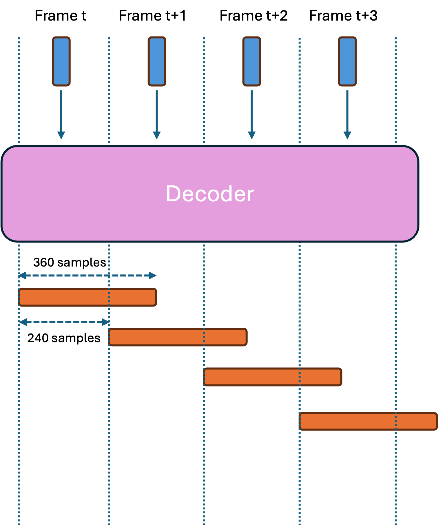
   Figure 1 Decoder using transposed convolutions with overlapping output frames and excess samples representing a prediction for future frames. In this case, upsampling operations do not create additional algorithmic latency to the system.

   • However, if the alignment of the input and the output audio, as well as the padding of the transposed convolution layers during training, is adjusted such that the last 240 samples of the L output samples correspond to the current input embedding, then we must wait for the next frames to finalize the overlap-add procedure for the current frame. This introduces additional algorithmic latency. An example of this case is depicted in Figure 2 with L=360. In this case, additional algorithmic latency of L-240 samples will be introduced. Note that we subtract encoder’s overall hop size of 240 samples here, similar to Example 3, because this portion is already accounted for in the buffering latency of the encoder.

   

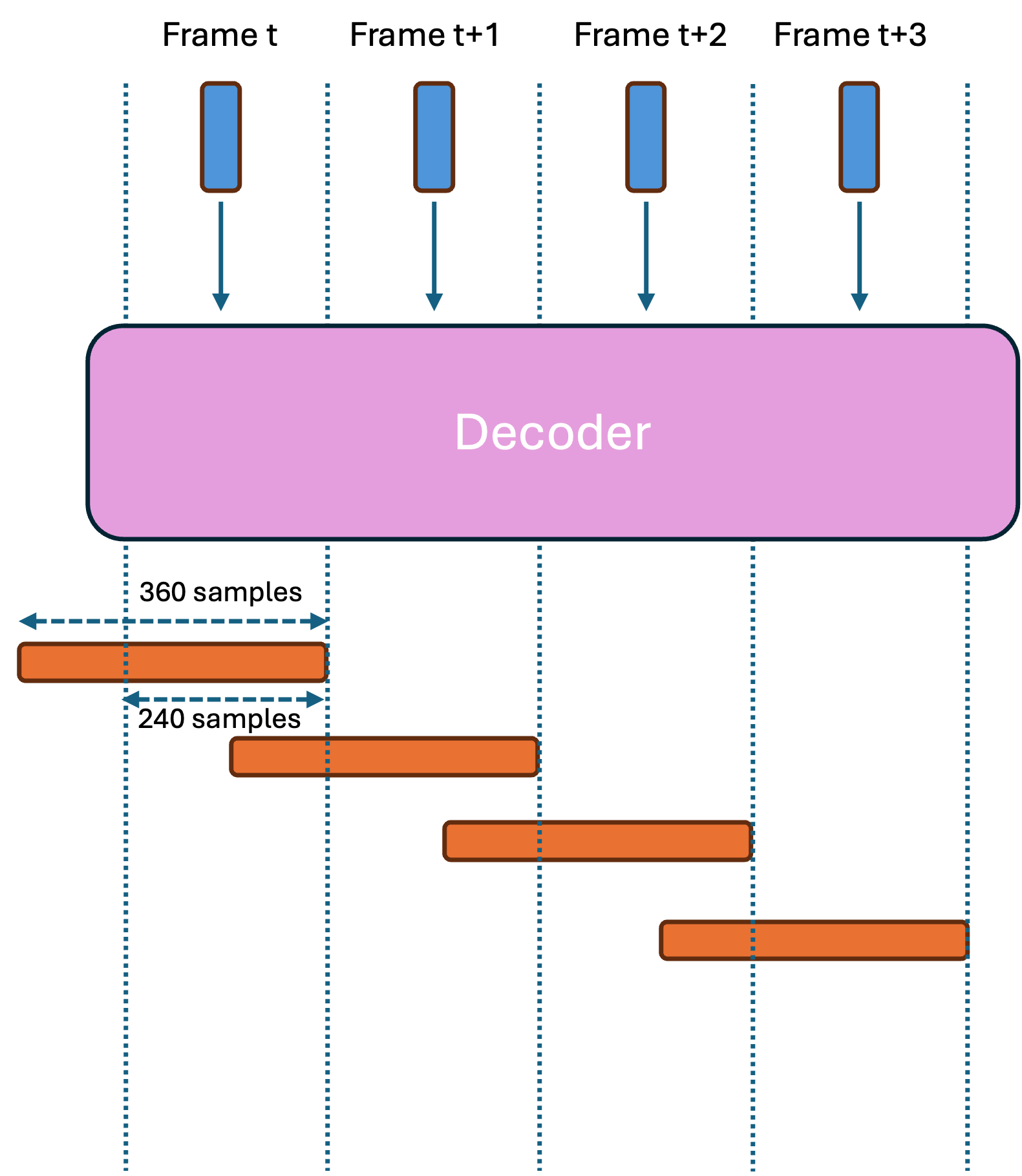
   Figure 2 Decoder using transposed convolutions with overlapping output frames and excess samples representing a prediction for past frames. In this case, upsampling operations create additional algorithmic latency to the system.

8. Inverse STFT as the last layer of a decoder network When inverse STFT is used as the last layer of a decoder network as in [3], it could be considered as a transposed convolution layer with fixed data-independent weights, and the same conditions of Example 7 apply in this case. Also see [4] for methods to reduce algorithmic latency of an encoder-decoder DNN architecture with STFT front-end and ISTFT upsampling.

References

1. N. Zeghidour, A. Luebs, A. Omran, J. Skoglund and M. Tagliasacchi, “SoundStream: An End-to-End Neural Audio Codec,” IEEE/ACM Transactions on Audio, Speech, and Language Processing, vol. 30, pp. 495-507, 2022, doi: 10.1109/TASLP.2021.3129994.
2. A. Défossez, J. Copet, G. Synnaeve and Y. Adi, “High fidelity neural audio compression”, Transactions on Machine Learning Research, 2023.
3. H. Siuzdak, “Vocos: Closing the gap between time-domain and fourier-based neural vocoders for high-quality audio synthesis”, arXiv preprint arXiv:2306.00814, 2023.
4. Z. Q. Wang, G. Wichern, S. Watanabe, and J. Le Roux, “STFT-domain neural speech enhancement with very low algorithmic latency”, IEEE/ACM Transactions on Audio, Speech, and Language Processing, vol. 31, pp. 397-410, 2022.

Back to top